Strong event contrasts
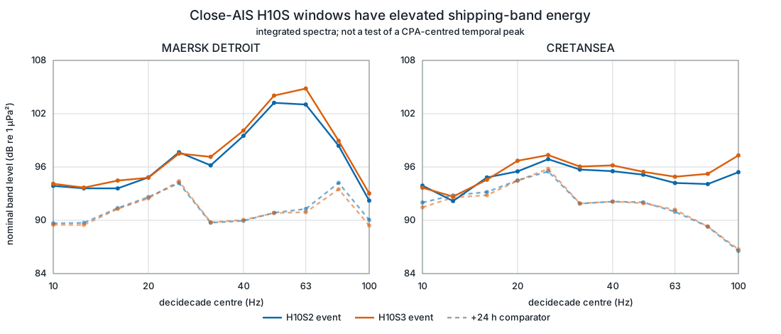
MAERSK DETROIT, CRETANSEA and Juan pair P3 have broad event-versus-comparison differences of roughly 6–15 dB in their strongest frequency ranges.
Several times selected from vessel data show broad acoustic rises on multiple hydrophones. Those event records merit targeted follow-up. They are not yet ship detections: their comparison records are weak, and complete three-hydrophone arrays have not repeatedly recovered the AIS bearings.
Automatic Identification System vessel data are useful for choosing hydroacoustic records to inspect, but the common 63 Hz ranking does not predict the size of the measured contrast. Four of six frozen high-versus-low pairs had the expected sign on every available node, while H08S reversed and H10N was near zero. A separate AIS-first direction test found no supporting case. None of these results identifies a ship as the cause.
MAERSK DETROIT, CRETANSEA and Juan pair P3 have broad event-versus-comparison differences of roughly 6–15 dB in their strongest frequency ranges.
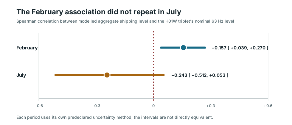
Across 561 exposed February hours, the modelled 63 Hz shipping screen and the measured triplet level have a rank correlation of +0.157. In a separately selected 46-hour July interval, the same frozen comparison gives −0.243 and an uncertainty interval that includes zero.
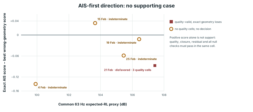
The newest complete-triplet pass selected five windows by AIS expected level alone. One was disfavored and four were indeterminate; none supported the AIS bearing. Ship contribution, attribution and prediction remain open.
The rest of this report explains exactly what an AIS row means, what was calculated from it, what the hydrophones measured, and why those pieces do not yet amount to attribution.
Automatic Identification System (AIS) messages describe a vessel’s reported position, time and, when present, speed, type and dimensions. The project uses three AIS-derived sources. They differ enough that their rows cannot be treated as interchangeable.
| Source | What one retained record means | How it is used here | What it cannot establish |
|---|---|---|---|
| Australian Maritime Safety Authority (AMSA) public monthly extracts | A public vessel-position report, thinned to at least hourly cadence and labelled with an anonymous CRAFT_ID. That identifier is not a Maritime Mobile Service Identity (MMSI) or an IMO ship number, and it is not assumed to persist across months. |
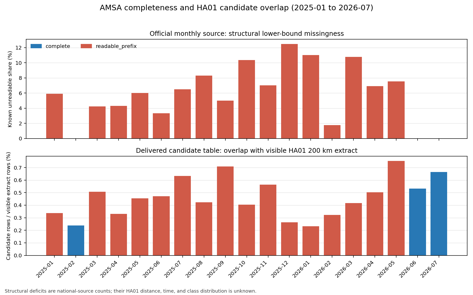
Traffic counts, anonymous passage screening, source-model inputs and the H01W candidate search. | A named vessel, an exact continuous track, or proof that a low-count hour had little traffic. Sixteen of the nineteen retained months are readable prefixes of files truncated at 2 GiB. |
| Locally held ARA regional exports | A row for one vessel with its own timeOfFix, inside an export that contains all rows delivered for a particular region and capture period. The files contain many vessels; they were not made by following one named ship. |
Exact named-vessel positions for the H10 and H08 cases after a row was selected from the regional export. | A continuous feed or a complete voyage. Capture times are irregular, rows may be carried forward, and the source network, extraction cadence and licence remain unresolved. “ARA” is retained as the project’s source label because the provider has not been established. |
| Global Fishing Watch (GFW) public presence | Approximately hourly, gridded vessel presence. | Independent class or identity context for some H10 rows and coarse traffic-bearing sectors at H08S and H10N. | A raw AIS message, an exact position, a continuous track or proof of vessel absence. |
The local contemporary ARA holding now covers eleven sparse station capture sets between 11 and 20 August: 43 valid CSVs with 7,254 source rows and 6,578 unique exact fixes. The three 20 August sets add 1,938 rows, but overlap no held waveform interval; their nominal 16 UTC files contain only positions at least 80 minutes old. None contains a true reported draught field. These files arrived after the common 63 Hz ranking below was sealed, so that ranking has not been silently changed.
Juan, a project collaborator, selected 678 AMSA rows in 233 Coordinated Universal Time (UTC) clock hours from nineteen monthly H01W extracts. His preliminary ranking used vessel class, size, speed, distance and a fast 63 Hz source-and-loss calculation. The project later matched all 678 rows back to the public source files, reconstructed their exact geometry and calculated direct transmission loss with the RAM parabolic-equation model at 63 and 80 Hz. Only forty rows, spread across twelve February 2026 hours, overlap the complete H01W waveform holdings used for the measured follow-up.
Before reading those measured acoustic contrasts, the project formed four non-overlapping high-versus-comparison pairs, called P1–P4. Within each pair, the comparison row has a lower modelled contribution and the same month-local anonymous CRAFT_ID. It is not a quiet period, a named-ship control or an environmentally matched control.
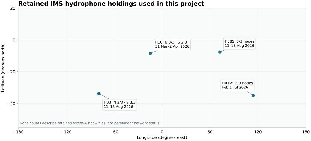
The International Monitoring System (IMS) hydroacoustic stations use separated underwater sensors. Labels such as H01W and H10S identify a station and array side; a final numeral identifies one sensor. H01W, H08S, H03S and H10N have complete three-node records for the periods held here, so arrival-time differences can in principle constrain direction. H03N has H03N1 and H03N2 but not H03N3. The H10S cases have only H10S2 and H10S3; H10S1 is absent. Those incomplete sides cannot supply a three-node bearing.
The archived waveform is a sequence of digitizer counts. Every retained waveform header also carries an exact-date WID2 CALIB value: the nominal pressure represented by one count at the stated CALPER. Here CALPER = 0.1 s, so the scalar is anchored at 10 Hz. For example, the H08S1 header states 542 µPa/count, while its full response gives 541.96 µPa/count at 10 Hz—a difference of 0.007%.
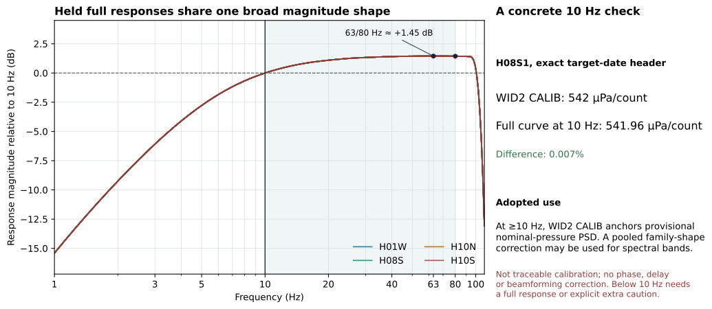
A full complex response describes both the frequency-dependent magnitude and phase. Where it is date-valid, using it produces a T1 nominal pressure spectrum. The project has now also adopted a pragmatic scalar-anchored convention for holdings without a date-valid full curve: at frequencies of 10 Hz and above, the WID2 scalar may be used to form provisional nominal-pressure spectral levels. At the central 63–80 Hz bands, either the pooled 1.45 dB magnitude correction is applied or a scalar-only result is reported with an approximately 1–1.5 dB response-shape bias. A scalar-only conversion is not T1 or traceable calibration, and it supplies no phase or delay correction for beamforming. It is not a safe shortcut below 10 Hz; the 5–10 Hz interval needs explicit caution.
A power spectral density (PSD) states mean-square pressure per hertz. The adopted convention now has a versioned derivative for H03N1–2, H03S1–3 and H10N1–3: 381 complete node-hours were recomputed from the immutable counts, producing provisional nominal-pressure bands from 12.5 through 100 Hz. The nominal 10 Hz decidecade was withheld because part of that band lies below the policy boundary. H01W, H08S and the selected H10S event spectra already use date-valid full responses and were not replaced.
The official International Data Centre (IDC) response for H03 has now been retrieved for the exact 11–13 August window and applied to the five nodes with waveform data; H03N3 still has no waveform. Across 2,400 hourly band values from 12.5 to 100 Hz, the official curve raises the earlier scalar-family estimates by about 0.05–0.63 dB. None changes by 1 dB. Seven comparisons change sign at 100 Hz only, where the compared values differ by no more than 0.04 dB; all lower-band signs are unchanged. The earlier scalar-anchored derivative remains a separate provisional version rather than being relabelled. This is a T1 nominal-pressure magnitude update, not traceable calibration, channel-health evidence or phase and delay correction. Recomputing the H10 event results with its official full response likewise changes retained summaries by at most about 0.02 dB and no reported sign, so the MAERSK and CRETANSEA interpretations remain unchanged.
The model does not predict the complete soundscape. It estimates the contribution from one AIS row under stated assumptions.
Source level (SL) is the JOMOPANS-ECHO estimate for a vessel of the reported class, length and speed. The standard production convention represents the ship as an equivalent monopole at 6 m depth. Transmission loss (TL) is the decrease in level predicted by the RAM parabolic-equation model along a specific path, frequency and ocean environment.
Thus an RLi value depends on the source equation, reported vessel state, frequency band, 6 m source-depth convention, ship position, bathymetry, water column, seabed and numerical grid. It excludes other ships and background sound. It is not the measured PSD and it is not ambient sound pressure level. When several ships are modelled, their unrelated contributions are added as linear power, not by adding decibels.
RAM is normally run from the station towards the reported ship position and interpreted by reciprocity. “Exact direct” in this report means that the calculation uses the row’s stated range and bearing, with complex pressure interpolated only across the final saved range bracket. It does not mean that the AIS feed supplies a complete track or that the ship was the acoustic source.
RAM can produce a precise number for a precisely stated path. The practical question is whether that number remains useful when ship depth, range, bearing or the ocean field is only approximately known. Four bounded tests now give a workable answer: keep exact-path RAM as the reference, show local sensitivities for important cases, and use interpolation or analytic loss laws only for screening inside their demonstrated limits.
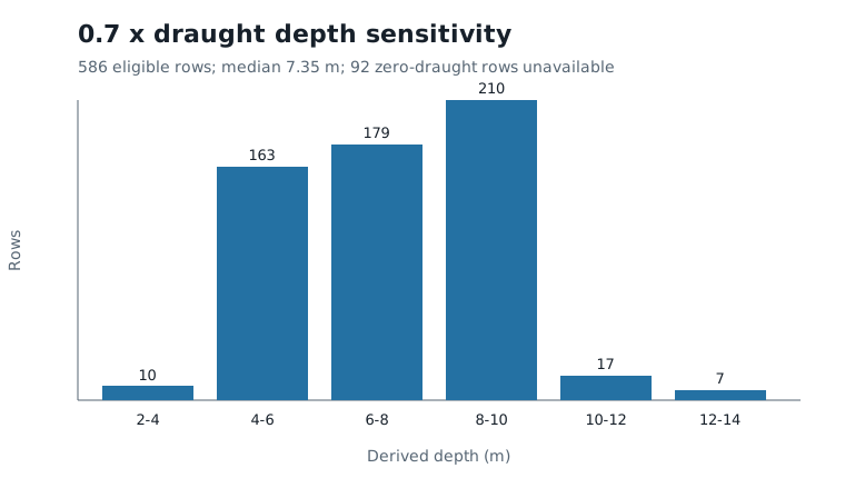
JOMOPANS-ECHO source levels are standardized to a 6 m equivalent-monopole depth, so production one-ship RLi values use 6 m TL. Of Juan’s 678 public AMSA rows, 586 have a finite positive reported draught. Their sensitivity depth, 0.7 × draught, ranges from about 2.7 to 13.3 m and has a median near 7.4 m; the remaining 92 rows contain a literal zero and are left unavailable.
Exact 63 and 80 Hz RAM at those alternate depths changes TL by a median of about −1.6 dB relative to 6 m, with individual differences from roughly −7.1 to +6.9 dB. Most paired high-versus-comparison contrasts change little because the two depth effects cancel; one P3 comparison at 80 Hz changes by about 3 dB.
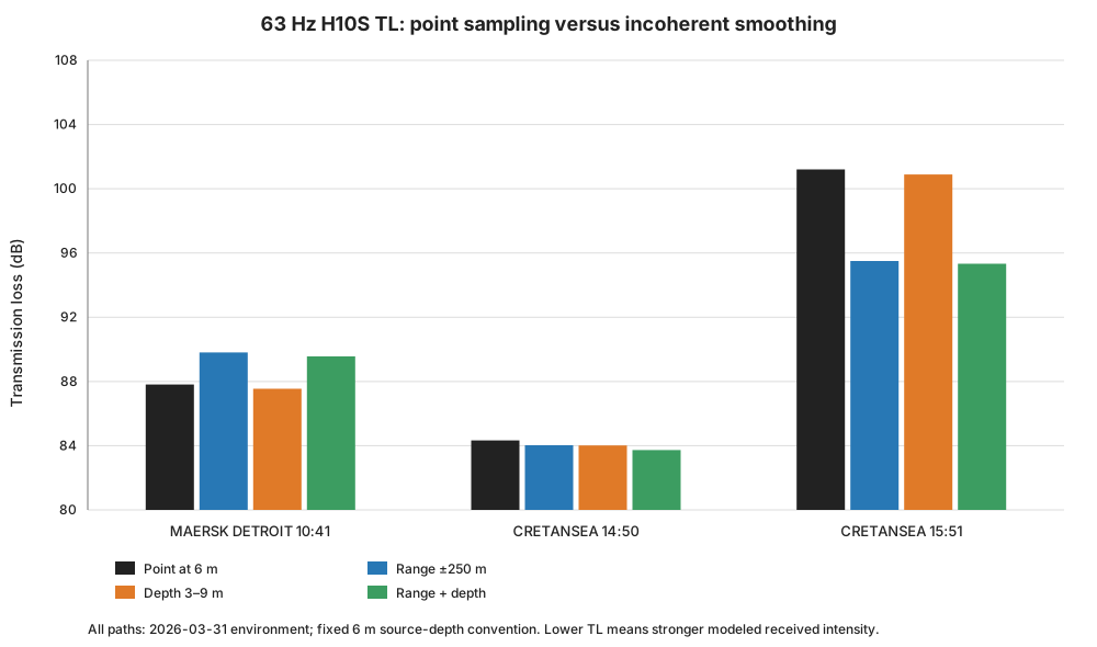
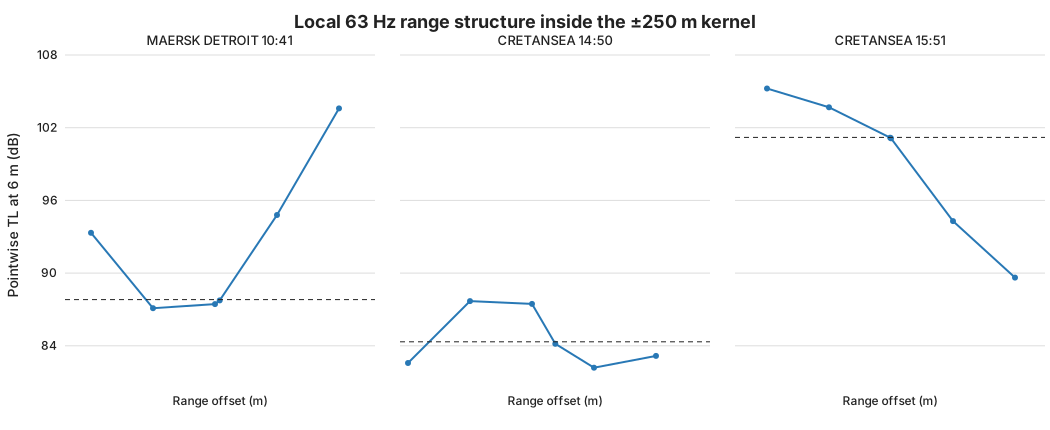
Three saved H10S fields were re-read at nominal 63 Hz with the fixed 6 m source depth and the 31 March daily ocean field. The point result was compared with incoherent intensity averages over ±250 m in range and 3–9 m in source depth. Depth averaging changed all three paths by only 0.26–0.31 dB. Range averaging changed CRETANSEA at 14:50 by 0.30 dB, MAERSK DETROIT by 2.00 dB, and CRETANSEA at 15:51 by 5.70 dB.
The 15:51 fix sits beside a sharp local range null: its point TL is about 101 dB, while the ±250 m intensity average is about 96 dB. The large point value is valid for the stated coordinate, but it is fragile to small position or path changes.
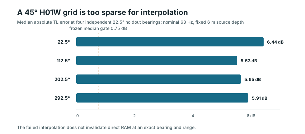
A separate H01W pilot calculated nominal 63 Hz, fixed-6 m fields on eight bearings spaced 45° apart, then withheld four halfway bearings from the interpolation. All thirteen direct fields were valid. Interpolation between the coarse anchors nevertheless missed the withheld fields by median absolute TL errors of about 5.5–6.4 dB; median phase errors were about 84–93°. Two directions also reach land or shallow water before the nominal 200 km limit.
The follow-up campaign calculated nominal 63 Hz fields on four five-degree tiles: one at H01W, one at H10N and two adjacent tiles at H10S. Each field stores a 50 m range grid and ship-side depths from 3 to 10 m. After the first 0.25° spacing failed, the frozen design allowed one refinement to 0.125° and two independent halfway bearings per tile. All 84 refinement rays completed, but every tile still missed the target of a median error no greater than 0.25 dB with at least 90% of ordinary samples within 0.5 dB.
| 63 Hz tile | Two holdout median errors | Samples within 0.5 dB |
|---|---|---|
| H01W | 0.58 / 0.69 dB | 47% / 43% |
| H10N | 0.38 / 0.38 dB | 58% / 57% |
| H10S, tile 36 | 0.63 / 0.62 dB | 45% / 46% |
| H10S, tile 37 | 0.74 / 0.74 dB | 43% / 43% |
Four outcome-blind H01W paths were recomputed at nominal 63 Hz and fixed 6 m depth with the calendar-month mean, the exact-date daily mean and the nearest six-hour ocean field. Daily-minus-monthly TL changes were −2.60, +3.66, +3.18 and +0.02 dB. Six-hour-minus-daily changes were +1.78, +0.41, −1.29 and −0.07 dB.
| Environment comparison | Four signed TL changes | Median absolute change | What it supports |
|---|---|---|---|
| Exact-date daily minus calendar-month mean | −2.60, +3.66, +3.18, +0.02 dB | 2.89 dB | Date choice can matter for a selected path. |
| Nearest six-hour field minus exact-date daily mean | +1.78, +0.41, −1.29, −0.07 dB | 0.85 dB | Sub-daily structure is sometimes material, but smaller in this pilot. |
The signs change from path to path, so no fixed offset can convert a monthly result into a daily or six-hour result.
The project now has one comparative ranking for 103,851 vessel–array rows from the retained AMSA and ARA data. Every row uses the published JOMOPANS-ECHO source model at nominal 63 Hz and the same simple range-only loss law. Mixing exact RAM for a few selected ships with an approximation for everyone else would distort the order, so exact RAM never changes this ranking.
The common loss law is Juan’s original TL_lite screen. With range r in metres and rkm in kilometres, it is:
The ranked quantity is source level minus TLlite. It is an expected single-vessel RL proxy, not a measured level. The law is neither tl_fast nor spherical spreading, and it is not RAM. It has no bearing, bathymetry, ocean environment or source-depth input. Its purpose is triage: apply one rough rule everywhere, then spend exact modelling or waveform effort on the most useful rows.
| Rank | Array | UTC | Anonymous AMSA CRAFT_ID | Range | Common 63 Hz RL proxy |
|---|---|---|---|---|---|
| 1 | H01W | 4 Oct 2025, 14:50:09 | 4765513744 | 12.4 km | 115.41 dB |
| 2 | H01W | 17 Jun 2025, 18:18:49 | 4552119639 | 7.7 km | 115.14 dB |
| 3 | H01W | 14 Apr 2025, 01:52:49 | 597855851 | 16.3 km | 111.66 dB |
| 4 | H01W | 25 Oct 2025, 15:21:19 | 4552119639 | 10.1 km | 111.35 dB |
| 5 | H01W | 27 Apr 2025, 07:20:22 | 1623730410 | 8.2 km | 110.42 dB |
All five are anonymous, hourly-thinned public AMSA fixes near H01W. Their exact coordinates and source inputs remain in the queryable table. They are shown here as a population-ranking example rather than as named candidate cases, so the table gives the relevant spatial context—array and range—instead of implying a reconstructed voyage on a case map. None has a retained overlapping waveform.
| Case | Common rank | Array | Common 63 Hz RL proxy | Separate exact-RAM diagnostic |
|---|---|---|---|---|
| Juan P3 high | 25 | H01W | 104.46 dB | Exact 63 Hz TL is 4.82 dB higher than TLlite |
| MAERSK DETROIT | 35 | H10S | 103.58 dB | Exact 63 Hz TL is 10.78 dB higher |
| Juan P1 high | 363 | H01W | 98.43 dB | Exact 63 Hz TL is 5.08 dB higher |
| Juan P2 high | 1,445 | H01W | 94.98 dB | Exact 63 Hz TL is 4.99 dB higher |
| CRETANSEA | 3,376 | H10S | 91.73 dB | Exact 63 Hz TL is 24.10 dB higher |
| Juan P4 high | 22,954 | H01W | 79.47 dB | Exact 63 Hz TL is 11.47 dB higher |
These exact-minus-common differences are diagnostics, not corrections to the rank. A positive value means RAM predicts more loss—and therefore a lower one-ship received level—than the common screen. Only 674 of 97,538 usable AMSA records and 5 of 3,591 usable ARA records have an existing exact 63 Hz direct path. Juan P3 at rank 25 is the first ranked row with a retained complete-triplet waveform overlap; the 24 rows above it are concrete future acquisition or analysis opportunities.
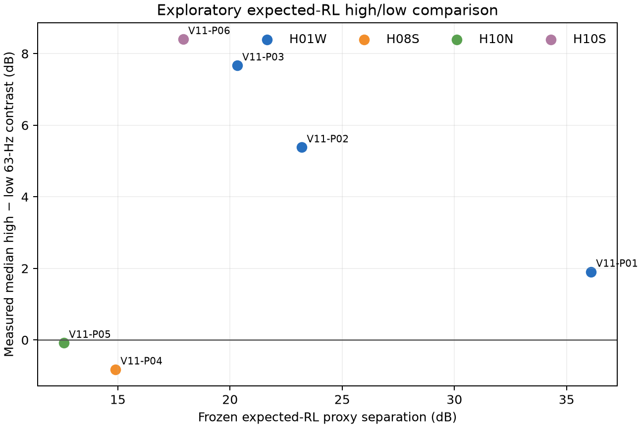
A separate outcome-blind screen selected six high-versus-low AIS pairs with retained waveforms. The common proxy predicted gaps of 12.6–36.1 dB. The measured 63 Hz high-minus-low contrasts were positive for all required nodes in four pairs: +1.91, +5.38 and +7.67 dB for the three H01W triplets, and +8.41 dB for the two-node H10S pair. H08S was −0.82 dB on the triplet median and negative on every node; H10N was −0.08 dB with one of three nodes positive.
The common proxy therefore remains useful for choosing cases, but not as a standalone acoustic predictor. Four of six pairs had the expected sign on every available node, yet the measured contrasts were far smaller than the predicted gaps. Across six non-independent pairs, the descriptive rank correlation was +0.37; the sample is too small and dependent for a significance claim. H03 supplied no pair because the ranked AIS rows did not overlap a retained H03 waveform.
The bar chart uses the retained eleven-band within-node median contrasts. Its inset places the high and low AIS fixes at their true bearings and ranges from the array; it does not reconstruct a voyage or closest point of approach. The exact coordinates and selection trail remain in the analysis package.
| Pair | Array coverage | Common proxy gap | Measured 63 Hz high − low | Node result |
|---|---|---|---|---|
| V11-P01 | H01W triplet | 36.09 dB | +1.91 dB | 3/3 positive |
| V11-P02 | H01W triplet | 23.20 dB | +5.38 dB | 3/3 positive |
| V11-P03 | H01W triplet | 20.32 dB | +7.67 dB | 3/3 positive |
| V11-P04 | H08S triplet | 14.90 dB | −0.82 dB | 0/3 positive |
| V11-P05 | H10N triplet | 12.60 dB | −0.08 dB | 1/3 positive |
| V11-P06 | H10S two nodes | 17.92 dB | +8.41 dB | 2/2 positive; no triplet bearing |
The complete queryable product and exact coverage table are described in the technical companion.
Once AIS had identified times worth examining, the acoustic question was simple to state: did the hydrophones become louder or acquire a repeatable spectral or directional structure at those times? The project attacked that question at three scales—individual events, repeated hours, and direction across a three-node array.
| Acoustic test | What was calculated | What appeared | What prevented a stronger conclusion |
|---|---|---|---|
| Event-versus-comparison energy | For fixed event and comparison windows, calculated power in standard non-overlapping frequency bands on each available hydrophone. The principal outputs are within-node decibel differences, which do not require absolute calibration. | MAERSK DETROIT, CRETANSEA, Juan P3, DIMIJOHN and several other selected events show broad positive differences on multiple nodes. P2 is a useful contrary case: its nominal comparison is stronger at high frequency. | Many comparisons are an unmatched time one day earlier or later. Other vessels, weather, geophysical arrivals and machinery-like sources can therefore explain part or all of a difference. |
| Spectra, spectrograms and tonal structure | Computed power spectral density, time–frequency plots, persistent narrowband lines, ridge continuity and node-to-node spectral agreement. Repeated fixed templates were then tested on other exposed periods. | The event leads are mostly broad 30–100 Hz rises. Several narrow lines recur within one scene or station period, including near 24–25 Hz, but fixed cross-time recurrence tests usually fail. A distinctive H10S harmonic comb is separable from the broad exact-traffic episode. | No narrow feature has remained both source-specific and repeatable. A line near a ship-selected time is not enough to identify shipping when the same or nearby frequency occurs in background records. |
| Repeated-hour association | Compared a modelled aggregate shipping-level predictor with H01W triplet energy across complete hours, within six-hour blocks and under fixed time-shift placebos. The same rule was then applied to a separately selected July record. | The February rank correlation was +0.157 across 561 exposed hours. In July it was −0.243 across 46 eligible hours, with all three nodes negative and an uncertainty interval that included zero. | The distinct-time reversal means the February relation cannot yet support prediction. Its strength also varies by UTC phase and is broadband rather than unique to 63 Hz. |
| Directional consistency | On complete triplets, tested time-delay closure, phase, beamforming, SRP-PHAT, spectral fingerprints, onset patterns and other scores. The newest pass selected five H01W windows by expected-RL rank alone, before reading direction or requiring a spectral line. | The AIS-first pass produced no directional support: one case was disfavored by the wrong-geometry controls and four lacked enough coherent cells to decide. | No tested real-data method repeatedly makes the AIS direction beat the alternatives. H10S event records have only two nodes, so they cannot produce a complete array bearing. |
| Alternative-source screening | Flagged strong transients and low-frequency event-like intervals, retained ambiguous moving-frequency structure, and compared traffic-selected H10S episodes with station boundaries, operations records and reviewed geophysical timing. | Five clear intervals were excluded from one directional development pool without changing its sign counts. A simple saved-record seam does not explain the main exact-traffic H10S episode. | Available metadata do not uniquely identify either H10S episode’s source class. Excluding too aggressively is also risky because a nearby ship can itself be transient. |
An earlier Family-C analysis first required a persistent horizontal spectral line, then required a timing-compatible AIS row, and only then compared the estimated acoustic direction with the AIS bearing. That design tested tonal candidates; it could not exclude non-tonal shipping. The new pass removed the tonal gate. It selected the five highest-ranked eligible H01W AIS rows from the 678-row screen, separated their receive centres by at least three hours, and retained every outcome.
| Direction method | What it uses | Used here? | Reason |
|---|---|---|---|
| Pooled 10–80 Hz spherical GCC-PHAT | Compares the three waveform time lags with delays predicted from the exact AIS point; requires pair coherence, delay closure, small residuals and wins over fixed wrong geometries. | Yes | Smallest existing complete-triplet AIS-conditioned estimator that could be applied identically to all five windows. |
| Full bearing/range SRP-PHAT scan | Searches a grid of candidate locations for lag agreement. | No | The fixed question concerned one AIS point; a full aliased search would add a different outcome. |
| HASE/PMCC/Bartlett | Fits far-field plane-wave arrival direction. | No | EDS/HASE/HAG execution remains unavailable; local PMCC was outside this frozen pass. |
| MVDR, phase-slope, onset and other development scores | Alternative beam, phase, onset or rank-fusion summaries. | No | Those development families had already been rejected or would create a new rescue score. |
| AIS emission time | Expected-RL proxy | AIS bearing | Coherence-quality cells | Strict AIS wins | Outcome |
|---|---|---|---|---|---|
| 21 Feb 2026 02:49:40 | 107.43 dB | 49.77° | 3/15 | 0/15 | Disfavored |
| 19 Feb 2026 05:29:56 | 106.44 dB | 67.14° | 0/15 | 0/15 | Indeterminate |
| 25 Feb 2026 03:09:57 | 105.45 dB | 64.63° | 0/15 | 0/15 | Indeterminate |
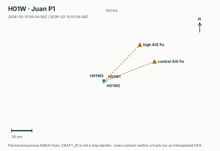
| 15 Feb 2026 00:04:58 | 103.66 dB | 44.80° | 0/15 | 0/15 | Indeterminate |
| 4 Feb 2026 18:14:58 | 99.92 dB | 64.30° | 0/15 | 0/15 | Indeterminate |
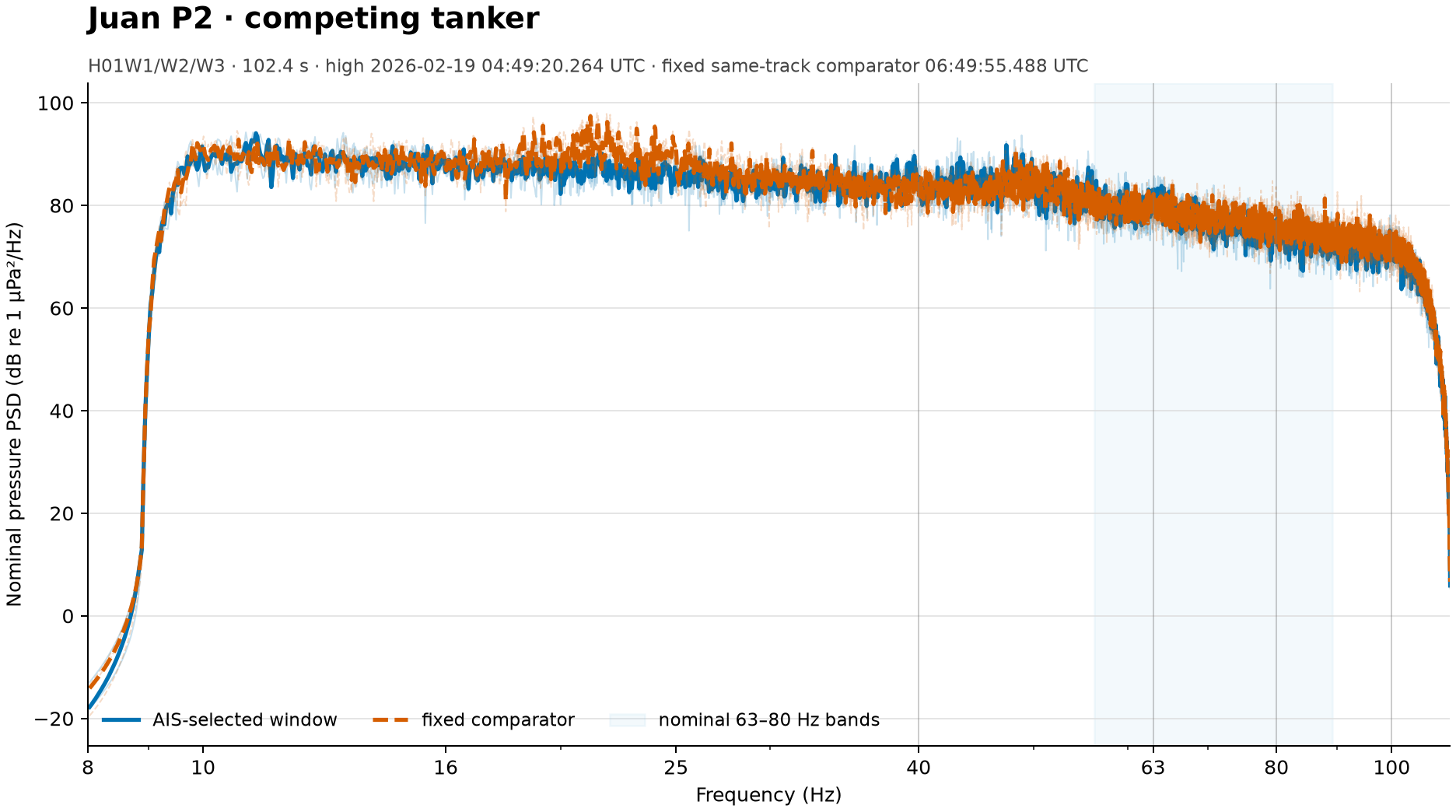
The selector below uses only saved, report-safe numeric products. Its upper panel shows the selected event or high-window PSD against its fixed comparison; its lower panel shows the saved target-minus-comparison band profile. It does not expose a complete hourly PSD or spectrogram atlas because those fine arrays were not retained for every analysis.
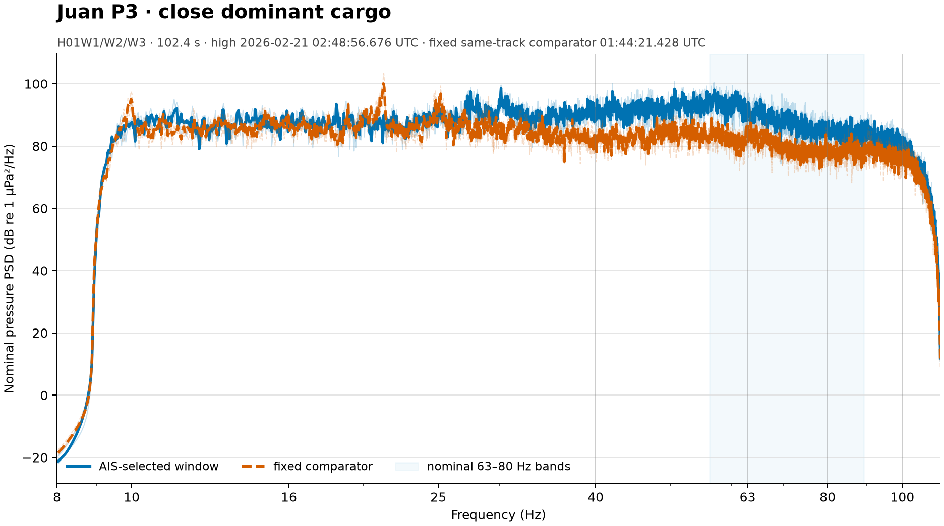
| Available selection | Station / channels | Retained comparison | Calibration basis |
|---|---|---|---|
| Juan P1, P2, P3 | H01W1–3 | 102.4 s AIS-selected high window versus fixed same-CRAFT_ID comparison | T1 nominal pressure; broad-Welch band summaries |
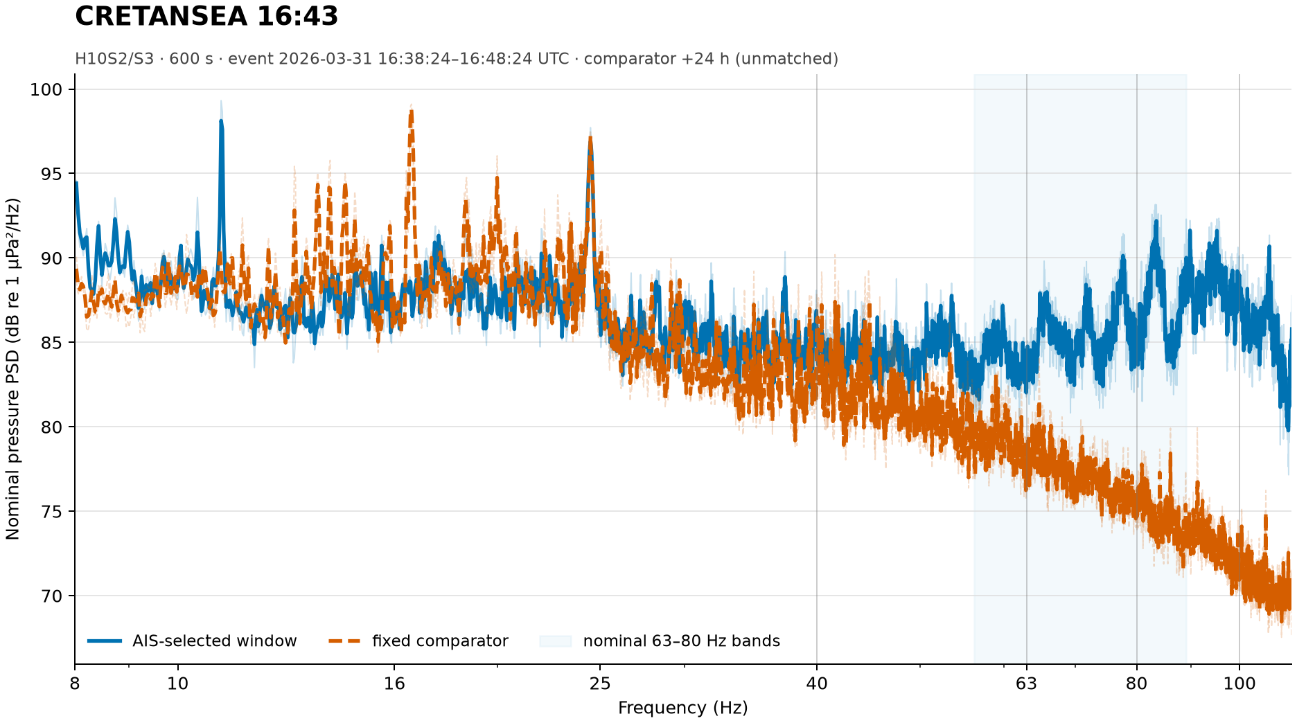
| MAERSK DETROIT; CRETANSEA 16:43 | H10S2–3 | 600 s selected event versus fixed unmatched +24 h window | T1 nominal pressure; H10S1 unavailable |
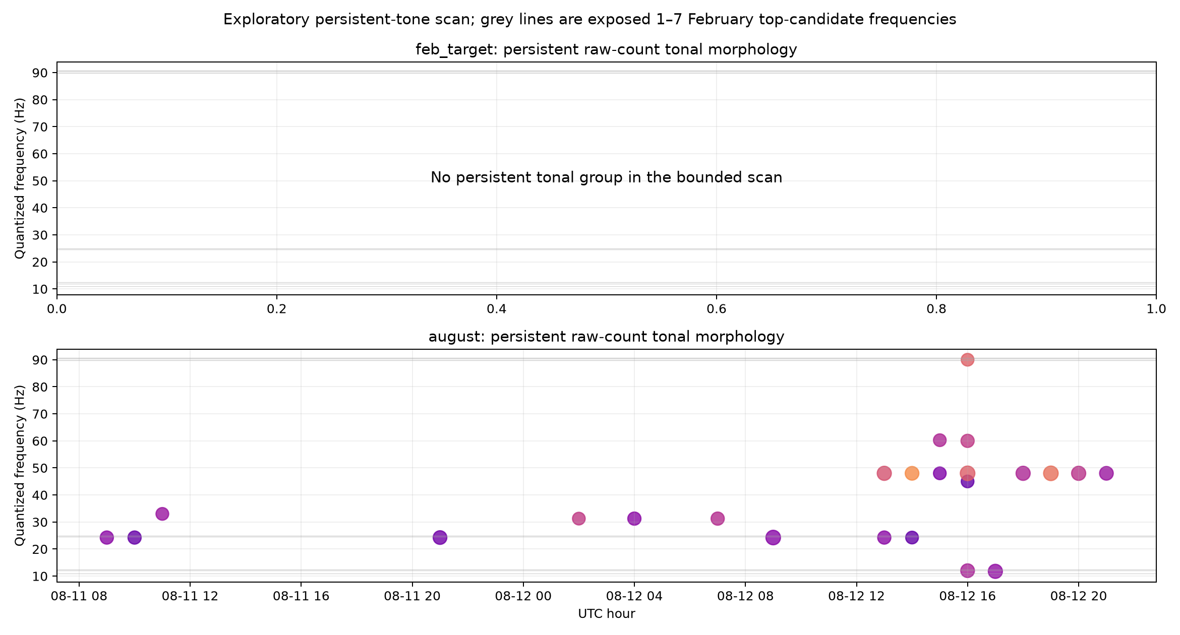
A separately frozen scan searched every eligible exposed full hour in the available H01W, H08S and H10N random-access packages. It covered 769 complete-triplet hours and excluded all 36 protected hours before reading their status or waveform values. The detector searched 10–100 Hz for a narrow peak at least 6 dB above its simultaneous local frequency background, present for at least half the hour with a continuous run of at least two minutes, and shared by at least two sensors.
| Array | Eligible hours | Hours with a supported narrow ridge | Within-hour families |
|---|---|---|---|
| H01W | 688 | 18 (2.6%) | 26 |
| H08S | 46 | 21 (45.7%) | 38 |
| H10N | 35 | 1 (2.9%) | 1 |
Overall, 40 of 769 hours contain 65 multi-node families. The concentration at H08S is a property of this exposed holding, not a station-rate estimate: its 21 positive hours come from one short interval. Several H08S lines lie between about 68.8 and 73.6 Hz on one date. A group near 48.16 Hz appears at both H01W and H08S, again on one date. The scan also finds near-29.85 Hz H01W lines, but those overlap already exposed source-scene material and do not alter the failed exact-frequency recurrence tests.
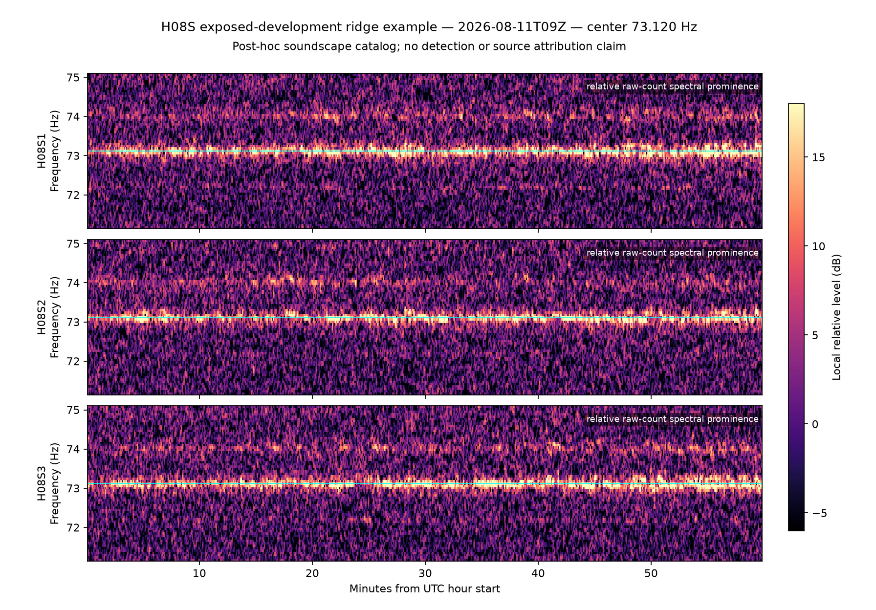
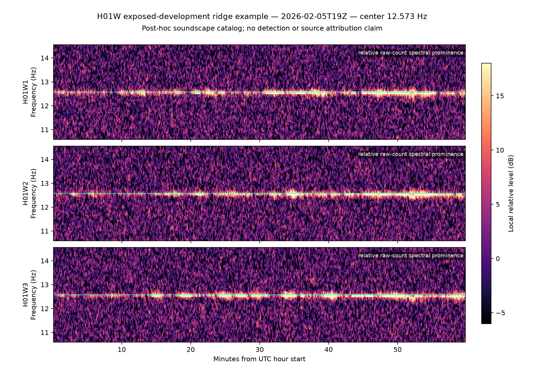
The earlier ten-minute H01W August scan remains a distinct local result. Under its stricter preselected rule, 48 Hz appeared in 8/47 hours, 24.25 Hz in 6/47 and 31.25 Hz in 3/47; none repeated in the separately frozen February test.
The next sections show the event records behind the strongest positive statements, followed by the population and direction results that limit those statements.
The technical companion gives the full method ledger; its station matrix records the available channels, dates and calibration tier.
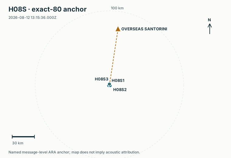
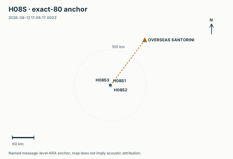
The maps below mark one selected timeOfFix row from an ARA regional export. The export contains many vessels and times; the dot is neither a reconstructed track nor the vessel’s closest point of approach.
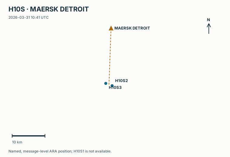
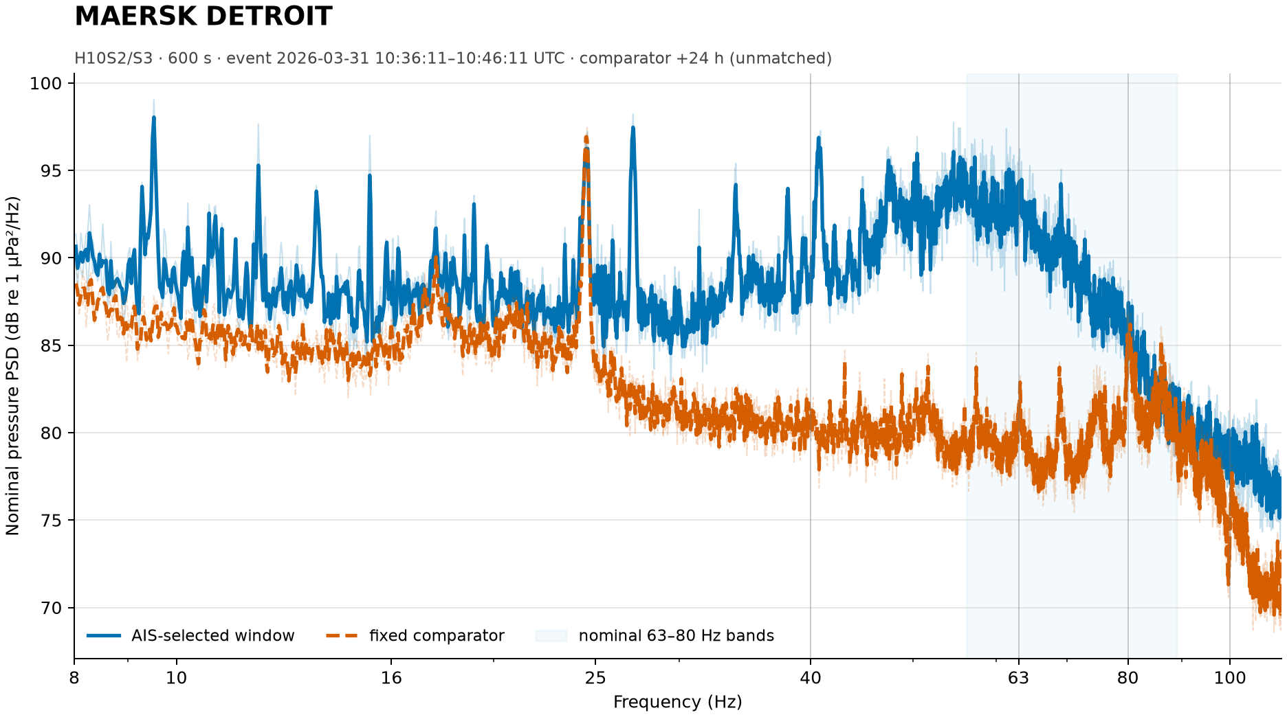
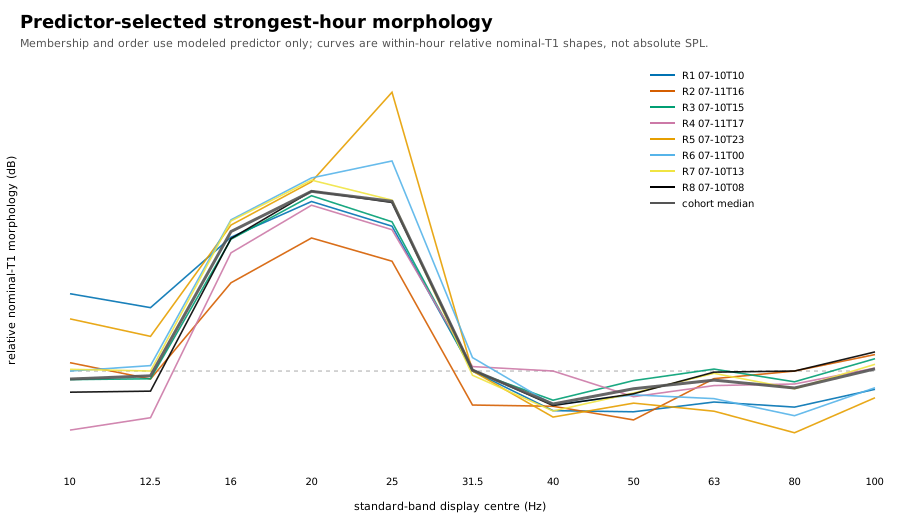
The fixed ten-minute event exceeds the same clock time one day later by about 10–12 dB across 40–80 Hz on both available H10S sensors.
The nominal-pressure PSD shows a broad rise rather than a unique machinery line. The +24-hour record was fixed in advance, but it was not shown to have similar weather, ocean state or traffic. This is the strongest two-node event morphology, not a ship detection.
Model context: nominal 63 Hz exact direct RAM, fixed 6 m ship-source depth and the 31 March daily ocean field give about 88 dB TL. Published JOMOPANS-ECHO SL minus that TL gives about 93 dB RLi for this one ship under those assumptions. Averaging intensity over ±250 m changes TL to about 90 dB; averaging over 3–9 m depth changes it to about 88 dB. None of these model values is the measured event PSD.
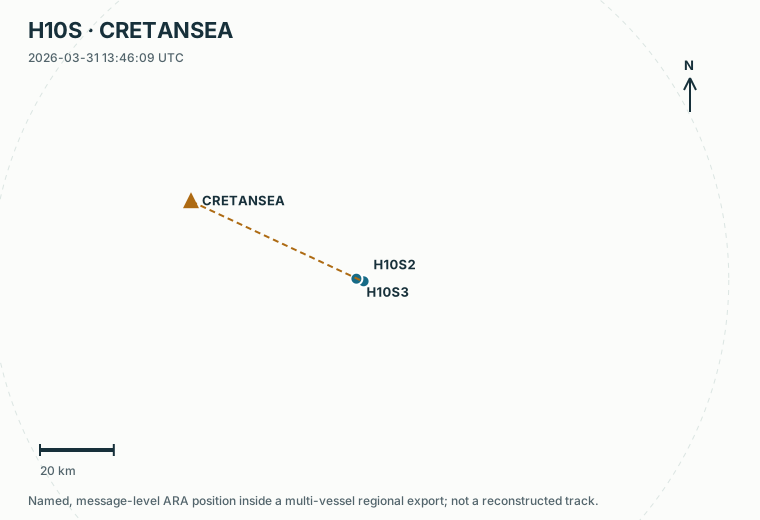
Exact direct RAM gives about 94 dB TL at 63 Hz and 86 dB at 80 Hz for the 50.5 km path.
The calculation uses the selected ARA position, the H10S centroid, the 31 March ocean field and the fixed 6 m ship-source depth. Published JOMOPANS-ECHO source level minus TL gives about 76 dB RLi at 63 Hz and 80 dB at 80 Hz. The corresponding receive time lies inside the previously inspected 13:40–14:00 broad-upper episode, but the regional AIS export contains several vessels and reviewed geophysical timing alternatives remain. The exact path adds model context; it does not identify CRETANSEA as the recorded source.
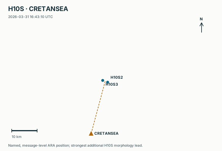
Both H10S sensors rise by about 7 dB over 40–80 Hz and by about 14–15 dB over 80–100 Hz.
The PSD confirms that the separation grows towards the top of the displayed range. The result still compares one previously inspected event with an unmatched +24-hour record, and H10S still lacks the third sensor needed for direction.
Model context: exact direct RAM at nominal 80 and 100 Hz, fixed 6 m ship-source depth and the 31 March ocean field gives about 89 dB TL at both frequencies. With the published Bulker source model, SL−TL is about 78 dB RLi at 80 Hz and 75 dB at 100 Hz. These are expected one-ship band levels, not measured ambient levels.
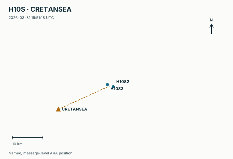
At nominal 63 Hz, fixed 6 m ship-source depth and the 31 March daily ocean field, the exact point gives about 101 dB TL. The propagation sensitivity section shows why this is a null-prone point value: averaging intensity over ±250 m lowers it by 5.7 dB, while averaging over 3–9 m depth changes it by only about 0.3 dB.
Heaney and colleagues describe short decidecade-level rises as a ship reaches its closest point of approach (CPA)—the time at which its distance to the receiver is smallest. Their illustrative analysis uses roughly 60-second observations around CPA and emphasizes 125 Hz. We have reviewed the H10S event spectra, but we have not reconstructed a continuous track and CPA for these ARA rows or calculated the same minute-by-minute statistic. The 250 Hz recordings also place 125 Hz at the Nyquist limit, the highest frequency they can represent without aliasing, rather than inside a normally analysed band. The broad H10S rises are compatible with Heaney’s qualitative picture; they are not yet a replication of that feature.
A separate source-class audit compared the 13:40–14:00 traffic episode with the comb-rich 07:20–08:00 episode on 1 April using retained station, acquisition, catalog, environment and traffic metadata rather than another acoustic score. It found no documented station change that uniquely explains either episode. The April comb ends at a routine record boundary, but adjacent H10S2 and H10S3 records are gapless and keep the same configuration. Both episodes also have reviewed geophysical timing alternatives. The retained metadata exclude a simple saved-record seam for the March episode and a gross three-hour surface-wave jump for the April episode; they do not select shipping or another source class.
These pairs come from the 678-row shortlist described in the data section. Their maps show two anonymous AMSA fixes—the model-selected “high” row and its lower-modelled comparison—not a continuous voyage or CPA. Every pair has exact direct H01W1 RAM at nominal 63 and 80 Hz using a fixed 6 m source depth and the February P1M calendar-month mean ocean field. Historical 63/80 Hz results remain preserved separately. The corrected current-master comparison uses the independently validated broad-run values at 63/80 Hz and exact current-master paths at 25, 40 and 100 Hz for P1, P3 and P4.
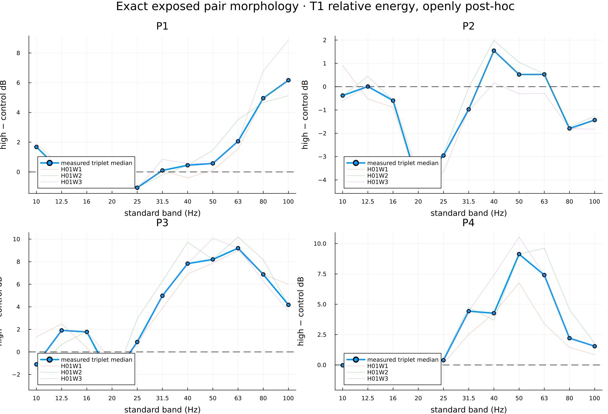
All three sensors are higher at 50, 63, 80 and 100 Hz; the broad analysis reaches about +6 dB at 100 Hz.
Across 25, 40, 63, 80 and 100 Hz, measured and modelled high-minus-comparison signs agree in three of five bands; they disagree at 25 and 100 Hz. The modelled and measured spectra peak in different bands, and their five-band rank correlation is −0.1. A near-30 Hz line recurs within this local scene but failed every later cross-time recurrence test. The frozen directional result is indeterminate, not a recovered AIS bearing.
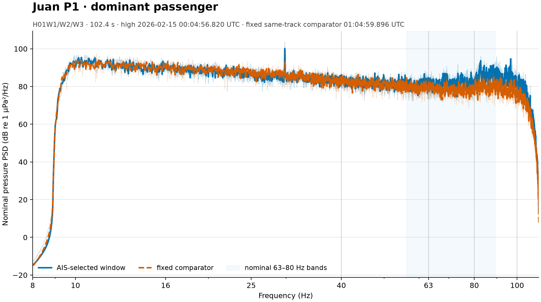
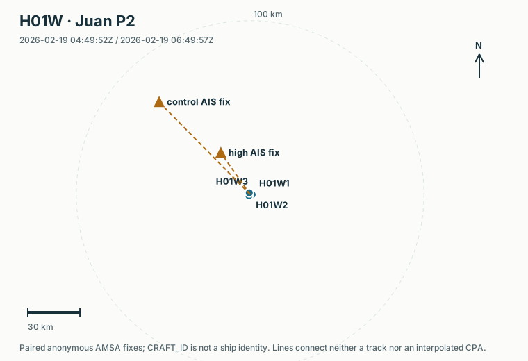
The measured difference is near zero at 63 Hz and reverses at 80 and 100 Hz.
The nominal “comparison” already contains elevated energy over much of 16–100 Hz. P2 is useful because it exposes the weakness of the control design: a lower modelled contribution for one anonymous row does not make the whole comparison soundscape quiet.
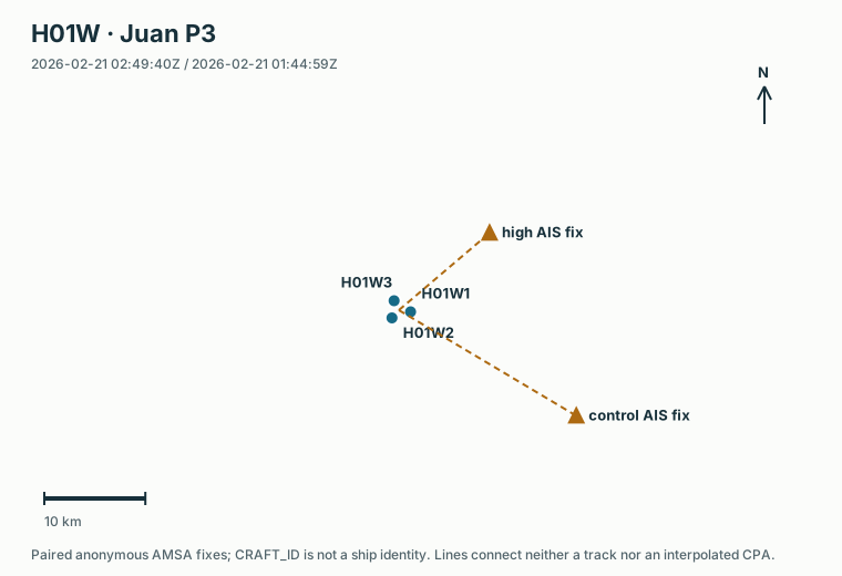
Nine of eleven standard bands are higher on every sensor; differences are roughly 4–9 dB from 31.5 to 100 Hz.
Across 25–100 Hz, measured and modelled signs agree in four of five bands; 100 Hz is the exception. Their peak bands differ and the five-band rank correlation is only +0.1. The frozen directional test passed its quality check but disfavoured the AIS geometry. P3 is therefore an energy-versus-direction stress case, not attribution.
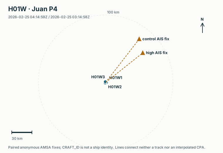
Measured and modelled signs agree in all five tested bands from 25 to 100 Hz, making P4 the broadest conditional ordering lead. They still peak in different bands, and their five-band rank correlation is only +0.3. A later search asked whether P4’s sharp 50 Hz-centred shape appears elsewhere without changing the definition. It appeared in 0 of 336 H01W hours, 0 of 40 eligible H08S hours and 0 of 41 H10N hours. This leaves the original P4 pair ordering intact, but rejects that exact sharp spectral shape as a repeated cross-station marker.
For a complete three-sensor array, a real coherent arrival should produce mutually consistent time delays between the three sensor pairs. The project tested delay-and-sum; steered-response power with phase-transform weighting (SRP-PHAT); minimum-variance distortionless-response beamforming (MVDR); and several phase, envelope and spectrotemporal scores. On real AIS-selected records, those methods did not repeatedly score the exact AIS geometry above fixed wrong directions and nearby times. This is why an energy rise does not yet become a directional ship result.
A separate comparison of previously inspected data asked an easier question: in a six-hour scene, is normalized directional acoustic energy larger in the sector containing more observed AIS traffic than in the opposite sector containing less observed traffic? The four maps below show the most promising selected examples. The displayed values are unitless score differences; positive values favour the traffic-richer sector and the target time. A low-observed sector is not a ship-free sector.
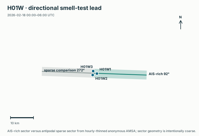
+0.111 richer versus poorer sector; +0.196 target versus nearby-time comparison.
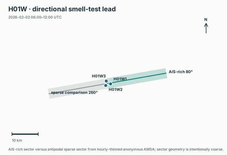
+0.075 richer versus poorer sector; +0.126 target versus nearby-time comparison.
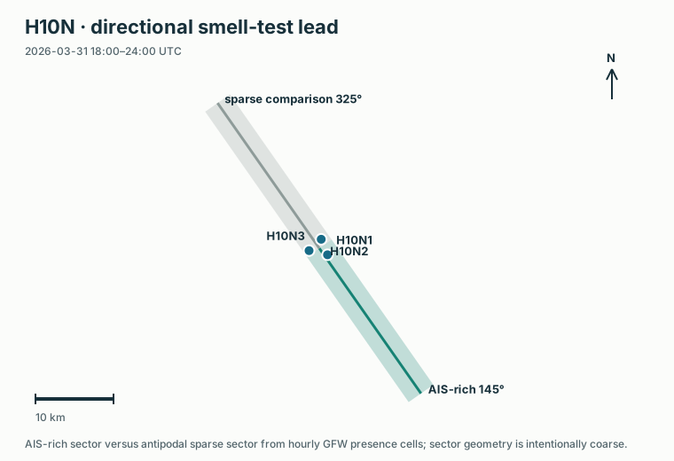
+0.014 richer versus poorer sector; +0.092 target versus nearby-time comparison.
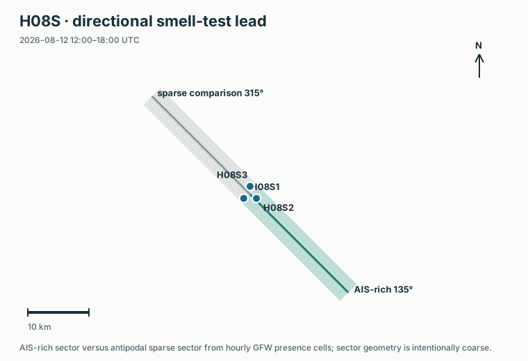
+0.086 richer versus poorer sector; +0.070 target versus nearby-time comparison.
The nineteen H01W extracts contain 159,925 readable AMSA rows within 200 km. The project assigned each row a nominal 63 Hz H01W1 transmission-loss value under the fixed 6 m source-depth convention and its same-calendar-month P1M ocean field. The method reused exact direct RAM at the 678 Juan anchor positions. It estimated other positions from nearby anchors in the same month.
The support is uneven: 17,442 non-anchor rows lie inside the polygon spanned by that month’s exact anchor positions, while 141,805 lie outside and are explicitly marked as extrapolations. With each anchor hidden in turn, the median absolute error is about 4 dB and the 95th percentile about 15 dB. The table is useful for deciding which positions deserve a new exact run. It is not exact RAM for all ships, and it contains no measured level or ship attribution.
A second step combined the 24,278 rows that pass Juan’s traffic gates into hourly modelled shipping-only levels. About 23,800 rows had usable speed and length. For each row, the calculation used corrected JOMOPANS source level, nominal 63 Hz H01W1 TL, fixed 6 m source depth, the same-month P1M ocean field, and travel time estimated as range divided by 1,500 m/s. Contributions from unrelated ships were summed in linear power.
The resulting 11,251 receive hours have an upper-bound median near 71 dB and a 95th percentile near 87 dB. The maximum, about 109 dB, occurs on 4 October 2025 at 14:00 UTC and comes from one anonymous cargo row with an exact TL anchor, about 12 km from H01W1. The top of the ranking has better spatial support than the full population: 64 of the top 100 hours include an exact anchor and 92 include at least one ship inside the anchor polygon.
These values are modelled shipping-only screening levels, not measured ambient SPL. Only 257 hours contain an exact anchor, 1,520 contain no ship inside the anchor polygon, the TL interpolation error is about 4 dB at the median and 15 dB at the 95th percentile, and the source model itself has roughly 6 dB scatter.
A prospectively fixed comparison joined the new predictor to 561 exposed, response-safe H01W triplet hours on 27 dates. The nominal-T1 63 Hz triplet level rises weakly but consistently with the modelled screen: Spearman correlation is +0.157, with a date-cluster interval from +0.039 to +0.270. After adjusting for date and UTC phase, one predictor interquartile range—about 13.4 dB—corresponds to only about +0.14 dB in the acoustic outcome, with an interval from +0.004 to +0.342 dB. All three sensors are positive, the within-six-hour-block correlation is +0.105, and the same-time relation is stronger than fixed +6, +24 and +168 hour future-predictor comparisons.
The relationship is not uniform. The 00–05 UTC phase has correlation +0.43, while the other three phases range only from +0.01 to +0.07; nine of fourteen two-day blocks are positive and five negative. This is the project’s first positive aggregate association based on the physical source-plus-path model, and it is stronger than the earlier fast range-loss screen. It remains an exposed February association, not a calibrated prediction or measured ship contribution.
A post-result robustness analysis shows that the February relationship is not caused by one date: all 27 leave-one-date-out correlations remain positive. The value nevertheless falls from +0.157 to +0.092 when the seven six-hour blocks containing exact model anchors are removed, and to +0.050 when the 00–05 UTC phase is removed. Every standard band from 10 to 100 Hz is positive both before and after removing six-hour-block means, so the pattern is broadband rather than peculiar to 63 Hz. This helps describe the lead; it does not validate it.
An August replication could not be run because the immutable modelled predictor ends on 31 July. The project therefore selected 10–12 July without inspecting its acoustic values, acquired all three H01W nodes and built a restricted triplet package. Each node is short by only its final 0.004-second sample; 47 of 48 triplet hours are complete, and the final hour was withheld rather than filled. No single ship map applies to this comparison because each predictor hour sums several anonymous AMSA rows; its spatial check is whether contributing positions lie inside the monthly RAM-anchor polygon.
The frozen July transfer uses 46 quality-eligible hours and reverses sign. Spearman correlation is −0.243, with an eight-block bootstrap interval from −0.512 to +0.053; the within-block correlation is −0.105 and all three sensors are negative. The +6-hour and +24-hour predictor comparisons are positive. Only one of eleven raw band associations is positive. Thus the February relationship did not transfer to this distinct interval. The result weakens any claim of a stable aggregate predictor, but it does not show that shipping sound is absent.
A post-result July atlas still found useful acoustic structure: a local 25 Hz maximum appears in 38 of the 46 eligible hours, including an eleven-hour run, and 11 July at 16:00 UTC is the strongest upper-frequency follow-up. A separately frozen arrival-time test at two high-modelled source clusters passed all four 50/63/80/100 Hz localization rules in 0 of 2 clusters; the second cluster passed only 50 and 63 Hz. Those are source-class leads, not a rescue of the failed aggregate transfer.
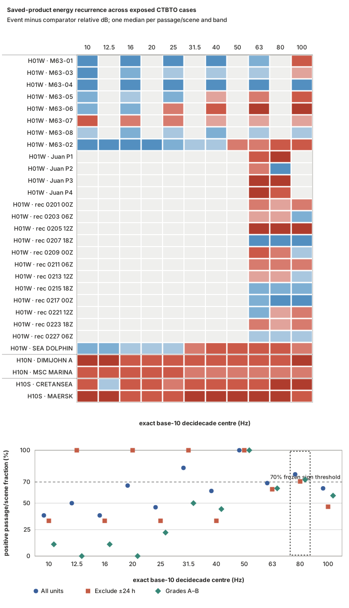
A saved-product synthesis combined 22 de-duplicated passage or scene comparisons from several stations. Exact 80 Hz was positive in 17 of 22. After removing comparisons that used an unmatched ±24-hour record, 12 of 17 remained positive. The strictest subset—restricted to the two higher preassigned comparator-quality grades and no ±24-hour record—was positive in 11 of 16, or 69%, just below its preset 70% screen.
A separate H08S check then applied fixed controls to two exact ARA rows. One was weakly positive and one negative; both control asymmetries were larger than the event differences. These two cases did not strengthen the recurrence lead.
Across 194 previously inspected H10S two-sensor ten-minute profiles, the fixed broad-upper shape appeared in 29 of 36 profiles previously selected for traffic or event analysis and in 67 of 158 other profiles. It also appeared in all three profiles previously described as machinery-like harmonic episodes. The shape therefore recurs in the acoustic data, but it cannot distinguish shipping from another machinery-like source.
A second fixed pass examined the same 194 profiles with much finer frequency bins. It retained 136 narrow ridges in 81 profiles. Only 12 of the 36 preassigned traffic/event profiles were ridge-positive, versus 69 of 158 other profiles; none of the three profiles with exact ARA traffic context contained a ridge. The known machinery-like harmonic episode was the only clearly comb-rich sequence. A component near 24.49 Hz appeared in 77 profiles and was therefore nonspecific. Fine spectra can recognize one machinery-comb morphology, but they do not yet supply a shipping marker.
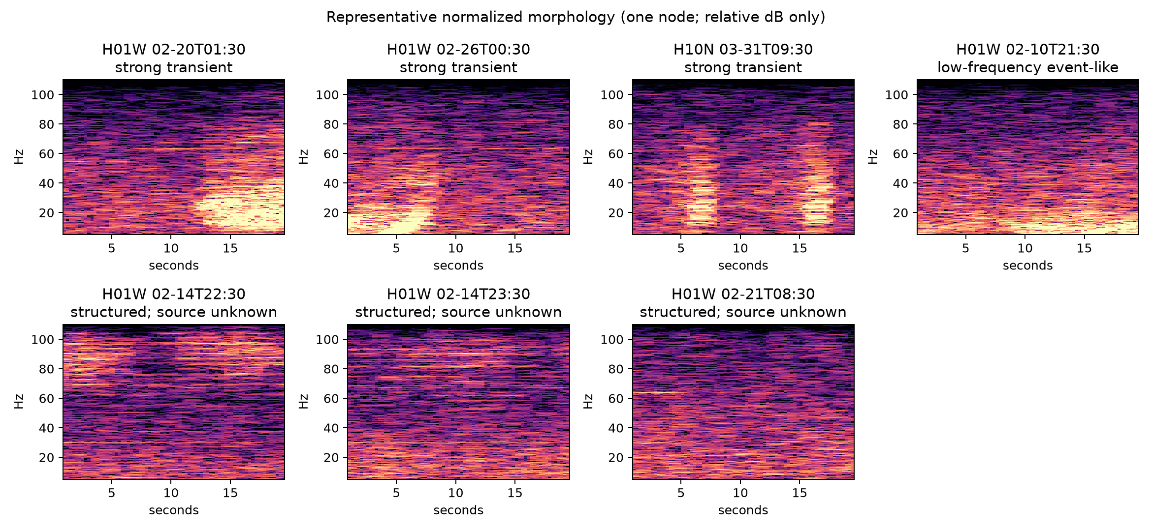
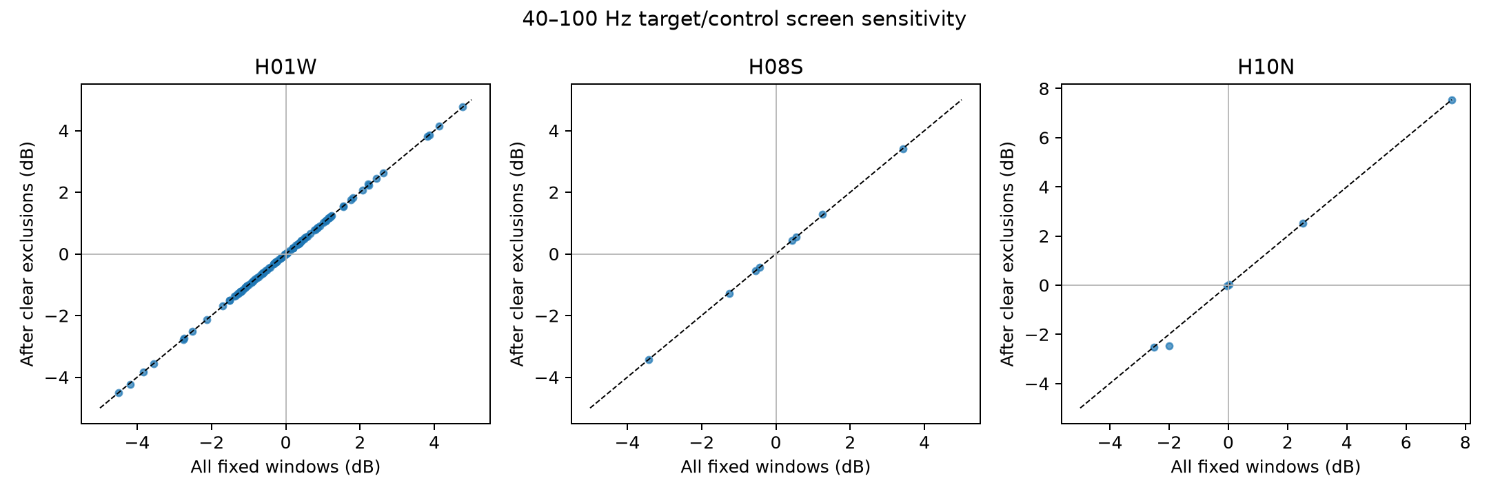
A conservative spectrogram review covered 732 unique previously inspected intervals. Five were clearly dominated by strong transient or low-frequency event-like structure and were excluded in a sensitivity branch. Three moving-frequency intervals were kept as “structured source unknown”; they were not labelled whales. Removing the five clear cases did not change the station-level positive counts in the 40–100 Hz screen.
For exact values, station coverage, calibration tiers, source-depth conventions, solver lineages and artifact paths, continue to the technical companion. The original 19 August report remains preserved.